MC Risking Analysis
Amrmoslim
April 23, 2019
Risking Analysis Using Monte Carlo Simulation
Input Data
library(mc2d)

### Inputs

  Tp90 <- 80       ### %      ### Trap MINIMUM VALUE
  Tp10 <- 90       ### %      ### Trap THROW MAXIMUM VALUE

  Rp90 <- 80       ### %      ### Reservoir MINIMUM VALUE
  Rp10 <- 90       ### %      ### Reservoir MAXIMUM VALUE

  Sp90 <- 80       ### %      ### Source MINIMUM VALUE
  Sp10 <- 90       ### %      ### Source MAXIMUM VALUE

  Mp90 <- 80       ### %      ### Migration MINIMUM VALUE
  Mp10 <- 90       ### %      ### Migration MAXIMUM VALUE
Data Processing (Creating Monte Carlo Model)
  n = 10000     ### NUMBER OF ITERATIONS
  seed = 999    ### SEED

  ### Calculate the SD
  Tsd <- sd(Tp90:Tp10)
  Rsd <- sd(Rp90:Rp10)
  Ssd <- sd(Sp90:Sp10)
  Msd <- sd(Mp90:Mp10)


  ### Calculate the Mean

  Tmean <- mean(Tp90:Tp10)
  Rmean <- mean(Rp90:Rp10)
  Smean <- mean(Sp90:Sp10)
  Mmean <- mean(Mp90:Mp10)

  ### Trap Distribution
  TR = mcstoc(rnorm, mean=Tmean, sd=Tsd, rtrunc=TRUE, linf=Tp90, lsup=Tp10, seed = seed, nsv= n )

  ###  Distribution
  Rs = mcstoc(rnorm, mean=Rmean, sd=Rsd, rtrunc=TRUE, linf=Rp90, lsup=Rp10, seed = seed, nsv= n )

  ### Source Distribution
  Sr = mcstoc(rnorm, mean=Smean, sd=Ssd, rtrunc=TRUE, linf=Sp90, lsup=Sp10, seed = seed, nsv= n)

  ### Source Distribution
  Mg = mcstoc(rnorm, mean=Mmean, sd=Msd, rtrunc=TRUE, linf=Mp90, lsup=Mp10, seed = seed, nsv= n)
  par(mfrow=c(2,2))
  #
  # hist(T, xlab="Fault throw (m)", breaks=100, col="cyan", border = NA)
  # hist(L, xlab="Layer Thickness (m)", breaks=100, col="red", border = NA)
  # hist(S, xlab="S (%)", breaks=100, col="yellow", border = NA)

  DENT <- density(TR)
  DENR <- density(Rs)
  DENS <- density(Sr)
  DENM <- density(Mg)
  plot(DENT, col="#ff606080", border=NA,xlab="Trap COS (%)",main = "Trap COS Distribution")
  polygon(DENT, col="#ff606080", border=NA)
  plot(DENR, xlab="Reservoir COS (%)",main = "Reservoir COS Distribution")
  polygon(DENR, col="#6060ff80", border=NA)
  plot(DENS, xlab="Source COS (%)",main = "Source COS Distribution")
  polygon(DENS, col="#bfff00", border=NA)
  plot(DENM, xlab="Migration COS (%)",main = "Migration COS Distribution")
  polygon(DENS, col="#FFDF9F", border=NA)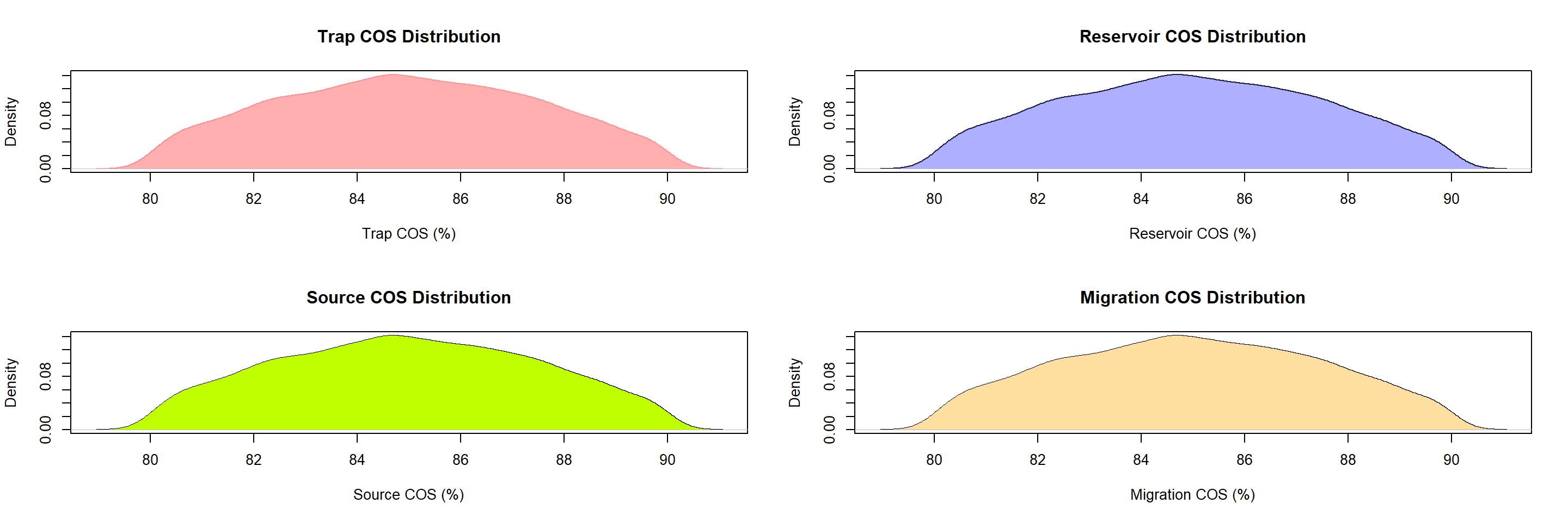
Results and Outputs
  GCOS = (TR/100 * Rs/100 *Sr/100 * Mg/100)*100

   ### Historgam plot for GCOS
   hist(GCOS, xlab="Geological Chance of Success (%)", breaks=100, col="seagreen1")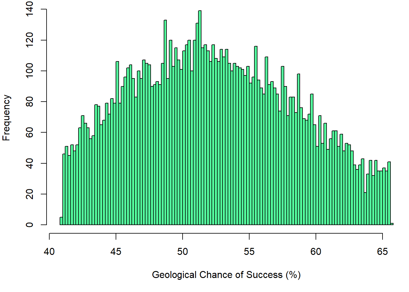
   ### density plot for GCOS
   DENGCOS <- density(GCOS)
   plot(DENGCOS)
        polygon(DENGCOS, col="#ff606080", border=NA)
        rug(GCOS, side = 3)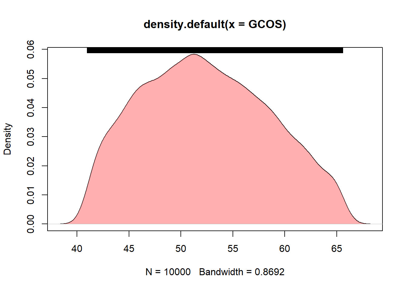
        #abline(v=c(18,22),lwd = 3,col = c("green","red") , lty =c(1,3))

   P<-summary(GCOS, probs = c(0.01,0.1,0.50,0.9,0.99))

   Pdata<- data.frame(unmc(P))
        colnames(Pdata)<- c("Mean","SD","1%","10%","50%","90%","99%")
        rownames(Pdata)[1] <- "GCOS"

knitr::kable(Pdata[1:7], digits = 0, caption = "GCOS MC Distribution ",booktabs = TRUE)| Mean | SD | 1% | 10% | 50% | 90% | 99% | |
|---|---|---|---|---|---|---|---|
| GCOS | 52 | 6 | 41 | 44 | 52 | 61 | 65 |
plot(x=c(1,10,50,90,99), y=Pdata[3:7], type="o",lwd = 3,
col="blue", main = "GCOS Probability Density Distribution",
xlab = "Distribution Percentages %",
ylab = "GCOS Distribution")
abline(v=c(10,50,90),lwd = 3,col = c("green","blue","red") , lty =c(1,2,3))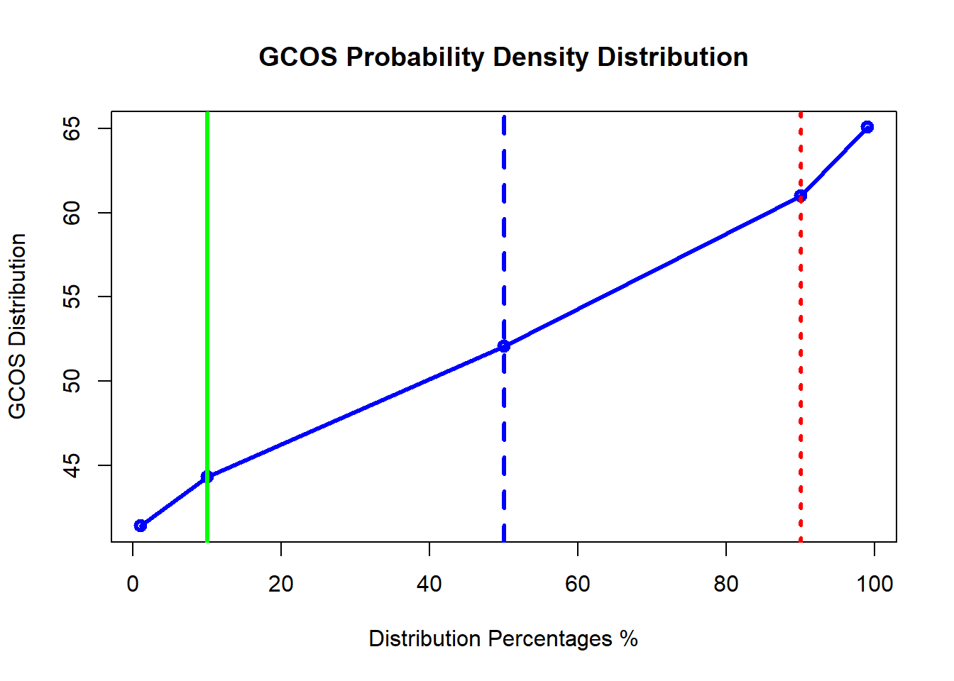 ############################################ Shinyapp has been created to calculate the risking analysis parameters without the hassel of changing the code. You can just play with the essential parameters and you get all the results instantaneously.
Please dont hesitate to contact me over a_moslim@live.com to share your comments.