1. Calculating the Discounted Cash Flow DCF
To understand the time value of Money for the two projects.
### Calculating the Discounted Cash Flow "DCF"
### the interest rate given is 0.06 "6%"

CDF.P1 <- dcf(Project1, r= 0.06, t0=TRUE)
cdfProject1<- data.frame(Time.Evaluation, Project1,CDF.P1)
knitr::kable(cdfProject1, digits = 2)
| 1 |
-1000 |
-1000.00 |
| 2 |
1250 |
1179.25 |
| 3 |
10 |
8.90 |
| 4 |
10 |
8.40 |
| 5 |
20 |
15.84 |
| 6 |
20 |
14.95 |
CDF.P2 <- dcf(Project2, r= 0.06, t0=TRUE)
cdfProject2<- data.frame(Time.Evaluation, Project2,CDF.P2)
knitr::kable(cdfProject2, digits = 2)
| 1 |
-1000 |
-1000.00 |
| 2 |
-10 |
-9.43 |
| 3 |
0 |
0.00 |
| 4 |
10 |
8.40 |
| 5 |
20 |
15.84 |
| 6 |
2000 |
1494.52 |
2. Claculating Net Present Value NPV
To understand the Whole project monetry value in the present day.
### NPV Calculations
npv.p1 <- npv(Project1, r=0.06, t0 = TRUE)
npv.p2 <- npv(Project2, r=0.06, t0 = TRUE)
npv.all <- data.frame(npv.p1,npv.p2)
knitr::kable(npv.all, digits = 2)
3. Calculating the Payback Period PBP
### PayBack Period Calculations
pbp.p1<- pbp(Project1)
pbp.p2<- pbp(Project2)
pbp.all <- data.frame(pbp.p1,pbp.p2)
knitr::kable(pbp.all)
dpbp.p1 <- dpbp(Project1, r= 0.06, t0=TRUE)
dpbp.p2 <- dpbp(Project2, r= 0.06, t0=TRUE)
dpbp.all <- data.frame(dpbp.p1,dpbp.p2)
knitr::kable(dpbp.all, digits = 2)
4. Calculating the Internal Rate Of Return IRR
### IRR Calculations
IRR.P1 <- irr(Project1)
IRR.P2 <- irr(Project2)
IRR.all <- data.frame(IRR.P1,IRR.P2)
knitr::kable(IRR.all, digits = 2)
##
## Attaching package: 'cowplot'
## The following object is masked from 'package:ggplot2':
##
##     ggsave
projects <- c("Project1","Project2")
NpvA <- c(npv.p1,npv.p2)
pay<- c(pbp.p1,pbp.p2)
dpay <- c(dpbp.p1,dpbp.p2)
ir <- c(IRR.P1,IRR.P2)
Econman <- data.frame(projects,NpvA, pay,dpay, ir)
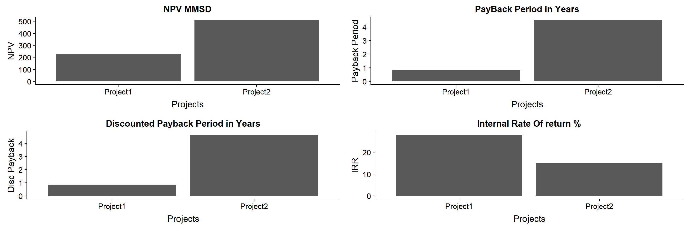
knitr::kable(Econman, digits = 2,caption = "The Economic parameters Comparison")
The Economic parameters Comparison
| Project1 |
227.33 |
0.80 |
0.85 |
0.28 |
| Project2 |
509.32 |
4.49 |
4.66 |
0.15 |
par(mfrow=c(2,2))
NPVPlt<- ggplot(data = Econman,aes(x=Econman$projects, y= Econman$NpvA))+geom_col()+labs(x = "Projects", y= "NPV", title = "NPV MMSD")
PayPlt<- ggplot(data = Econman,aes(x=Econman$projects, y= Econman$pay))+geom_col()+labs(x = "Projects", y= "Payback Period", title = "PayBack Period in Years")
dpayPlt<- ggplot(data = Econman,aes(x=Econman$projects, y= Econman$dpay))+geom_col()+labs(x = "Projects", y= "Disc Payback", title = "Discounted Payback Period in Years")
IRRPlt<- ggplot(data = Econman,aes(x=Econman$projects, y= Econman$ir*100))+geom_col()+labs(x = "Projects", y= "IRR", title = "Internal Rate Of return %")

plot_grid(NPVPlt,PayPlt,dpayPlt,IRRPlt)
Shinyapp has been created to estiamte the economic analysis of any given projects without the hassel of changing the code. You can just play with the essential parameters and you get all the results instantaneously.
Please dont hesitate to contact me over a_moslim@live.com to share your comments.