Fault Seal Analysis

AmrMoslim

2019-04-24

R Fault Seal Analysis Usong R “FSAR”

R Fault Seal Analysis Usong R “FSAR”

The most two famous and common processes to determine the fault seal analysis are Shale Gouge Ratio “SGR” and Shale Smear Factor “SSF”.

Data Input

library(mc2d)

### Inputs
  
  Ftp90 <- 120    ### Meters ### FAULT THROW MINIMUM VALUE
  Ftp10 <- 1000   ### Meters ### FAULT THROW MAXIMUM VALUE
  
  Ltp90 <- 140    ### Meters ### LAYER THICKNESS MINIMUM VALUE
  Ltp10 <- 500    ### Meters ### LAYER THICKNESS MAXIMUM VALUE
  
  Ngp90 <- 20     ### %      ### NET OVER GROSS MINIMUM VALUE
  Ngp10 <- 60     ### %      ### NET OVER GROSS MAXIMUM VALUE

Data Processing (Creating Monte Carlo Model)

  n = 10000     ### NUMBER OF ITERATIONS
  seed = 999    ### SEED 
  
  ### Calculate the SD 
  Ftsd <- sd(Ftp90:Ftp10)
  Ltsd <- sd(Ltp90:Ltp10)
  ngsd <- sd(Ngp90:Ngp10)
  
  ### Calculate the Mean 
  
  Ftmean <- mean(Ftp90:Ftp10)
  Ltmean <- mean(Ltp90:Ltp10)
  ngmean <- mean(Ngp90:Ngp10)

  ### Fault throw Distribution
  Ft = mcstoc(rnorm, mean=Ftmean, sd=Ftsd, rtrunc=TRUE, linf=Ftp90, lsup=Ftp10, seed = seed, nsv= n )

  ### Layer thickness Distribution
  Lt = mcstoc(rnorm, mean=Ltmean, sd=Ltsd, rtrunc=TRUE, linf=Ltp90, lsup=Ltp10, seed = seed, nsv= n )
  
  ### NG Distribution
    NG = mcstoc(rnorm, mean=ngmean, sd=ngsd, rtrunc=TRUE, linf=Ngp90, lsup=Ngp10, seed = seed, nsv= n)
  par(mfrow=c(1,3))
  # 
  # hist(Ft, xlab="Fault throw (m)", breaks=100, col="cyan", border = NA)
  # hist(Lt, xlab="Layer Thickness (m)", breaks=100, col="red", border = NA)
  # hist(NG, xlab="NG (%)", breaks=100, col="yellow", border = NA)
  
  DENFT <- density(Ft) 
  DENLT <- density(Lt)
  DENNG <- density(NG)
  plot(DENFT, col="#ff606080", border=NA,xlab="Fault throw (m)",main = "Fault Throw Distribution") 
  polygon(DENFT, col="#ff606080", border=NA)
  plot(DENLT, xlab="Layer Thickness (m)",main = "Layer Thickness Distribution")
  polygon(DENLT, col="#6060ff80", border=NA)
  plot(DENNG, xlab="NG (%)",main = "Net/Gross Distribution")
  polygon(DENNG, col="#FFDF9F", border=NA)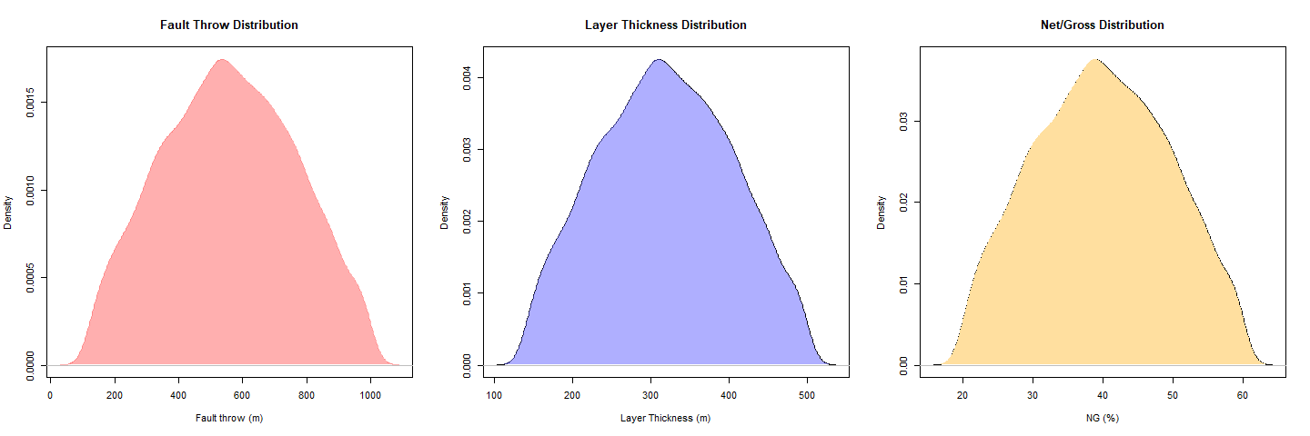

Results and Outputs

Shale Gouge Ratio Claculation

  SGR = (((100-NG)*Lt/Ft))
  
   ### Historgam plot for SGR
   hist(SGR, xlab="SGR (%)", breaks=100, col="seagreen1")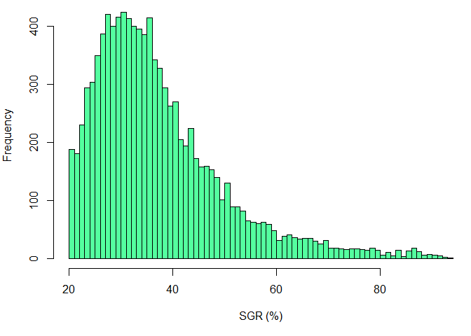

   ### density plot for SGR
   DENSGR <- density(SGR)
   plot(DENSGR) 
        polygon(DENSGR, col="#ff606080", border=NA)
        rug(SGR, side = 3)
        abline(v=c(18,22),lwd = 3,col = c("green","red") , lty =c(1,3))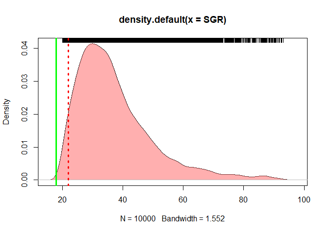

   P<-summary(SGR, probs = c(0.01,0.1,0.50,0.9,0.99))
   
   Pdata<- data.frame(unmc(P))
        colnames(Pdata)<- c("Mean","SD","1%","10%","50%","90%","99%")
        rownames(Pdata)[1] <- "SGR"
        
        SGRdata <- as.data.frame(Pdata[3:7])
   
   knitr::kable(Pdata[,1:7], digits = 0,  caption = "SGR MC Distribution ",booktabs = TRUE)

SGR MC Distribution
	Mean	SD	1%	10%	50%	90%	99%
SGR	37	13	21	24	34	54	82

   plot(x=c(1,10,50,90,99), y=Pdata[3:7], type="o",lwd = 3,
            col="blue", main = "SGR Probability Density Distribution",
           xlab = "Distribution Percentages %",
           ylab = "SGR Distribution")
            abline(v=c(10,50,90),lwd = 3,col = c("green","blue","red") , lty =c(1,2,3))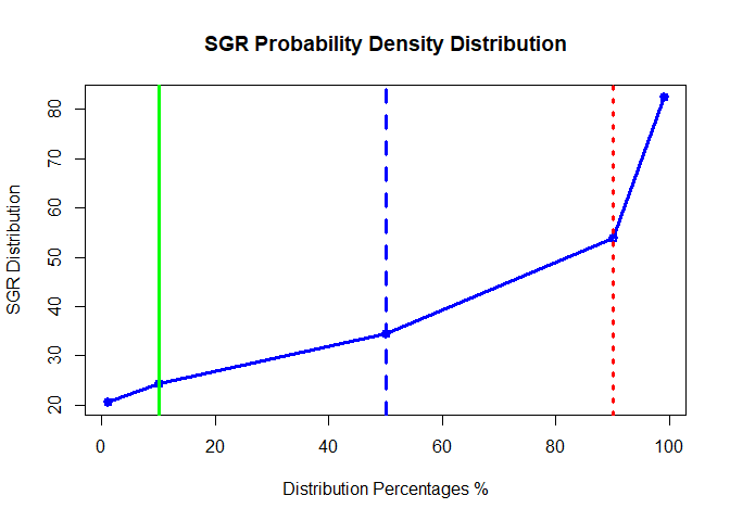

Shale Smear Factor Claculation

  SSF = (Ft/((100-NG)*Lt))*100

    ### Histogram plot for SSF
  hist(SSF, xlab="SSF (%)", breaks=100, col="orange")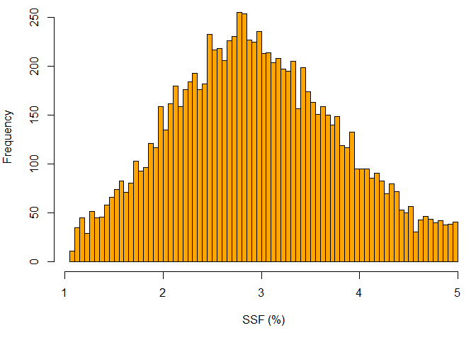

    ### density plot for SSF
   DENSSF <- density(SSF)
   plot(DENSSF) 
        polygon(DENSSF, col="#ff606080", border=NA)
        rug(SSF, side = 3)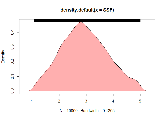

  SSFP<-summary(SSF, probs = c(0.01,0.1,0.50,0.9,0.99))
  PSSFdata<- data.frame(unmc(SSFP), drop= TRUE)
  
  colnames(PSSFdata)<- c("Mean","SD","1%","10%","50%","90%","99%")
  rownames(PSSFdata)[1] <- "SSF"
     SSFy5 = list(PSSFdata[3:7])
    
     knitr::kable(PSSFdata[,1:7], digits = 0,  caption = "SSF MC Distribution ",booktabs = TRUE)

SSF MC Distribution
	Mean	SD	1%	10%	50%	90%	99%
SSF	3	1	1	2	3	4	5

   plot(x=c(1,10,50,90,99), y=PSSFdata[3:7], type = "o",col="red",lwd = 3, main = "SSF Probability Density Distribution",
           xlab = "Distribution Percentages %",
           ylab = "SSF Distribution") 
            abline(v=c(10,50,90),lwd = 3,col = c("green","blue","red") , lty =c(1,2,3))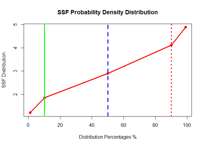

References

Shinyapp has been created to calculate FSA Parameters automatically without the hassel of changing the code. You can just play with the essential parameters and you get all the results instantaneously.

Please dont hesitate to contact me over a_moslim@live.com to share your comments.